**Assignment 2 : Single View to 3D** **Author:** *Rishikesh Jadhav (119256534)* Exploring Loss Funtions ================ Fitting a Voxel Grid ------------------------   ### Implementation Note The goal is to make a 3D binary voxel grid closely match a target voxel grid. We use a Binary Cross-Entropy loss to measure the difference between the two grids. It optimizes the source grid iteratively to minimize this loss, squashing its values using the sigmoid function. The result is a source voxel grid that aligns with the target. Fitting a Point Cloud ------------------------   ### Implementation Note The goal is to align a 3D point cloud with a target point cloud. We do this by finding the nearest neighbors between points in the source and target clouds and using the Chamfer distance as a measure of difference. Optimization updates the source point cloud to minimize this distance, making it match the target point cloud. Fitting a Mesh ------------------------   ### Implementation Note The goal is to fit a 3D mesh to a target mesh. Optimization updates the vertices of the source mesh to align with the target mesh. Two loss components are used: Chamfer Loss, to match points sampled from both meshes, and Smoothness Loss, which encourages the source mesh to have a smooth surface. The result is a source mesh closely matching the target. Reconstructing 3D from single view ================ Image to Voxel Grid ------------------------          ### Implementation Note The Voxel Decoder architecture is designed with a series of decoder blocks, each performing convolution, batch normalization, and optional ReLU activation. The final layer transforms the processed features into the predicted binary voxel grid. The decoder efficiently converts encoded image features into binary voxel grids, integral to the successful transformation of 2D images into 3D voxel representations. Image to Point Cloud ------------------------          ### Implementation Note The Point Cloud Decoder is tailored for the task of generating point clouds from encoded features. It comprises a sequence of fully connected layers with ReLU activations, culminating in a layer that produces point coordinates. The network takes encoded image features and reshapes the output into point clouds, enabling the transformation of encoded image data into 3D point clouds. Image to Mesh ------------------------          ### Implementation Note The Mesh Decoder is specifically designed for generating 3D meshes from encoded features. It consists of a sequence of fully connected layers with ReLU activations, concluding with a layer that produces vertex coordinates. The network takes encoded image features and reshapes the output into mesh vertices, enabling the transformation of encoded image data into 3D mesh representations. Quantitative Comparisions ------------------------    **Explanation :** It's worth noting that the difference between mesh and point cloud predictions and graphs is quite minimal, as observed in the results in the above section. One possible reason for the higher score in point cloud predictions could be the utilization of a significantly larger number of data points (n_points). On the other hand, the regularization applied during mesh training might impose constraints that slightly hinder its performance. Additionally, the voxel ground truth data has a lower resolution compared to the point cloud ground truth, and this disparity in resolution is likely affecting the performance of voxel predictions. 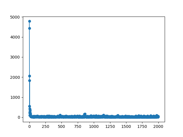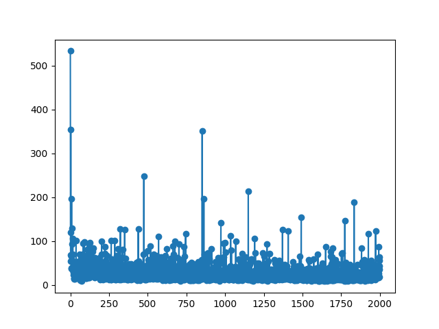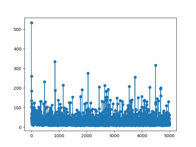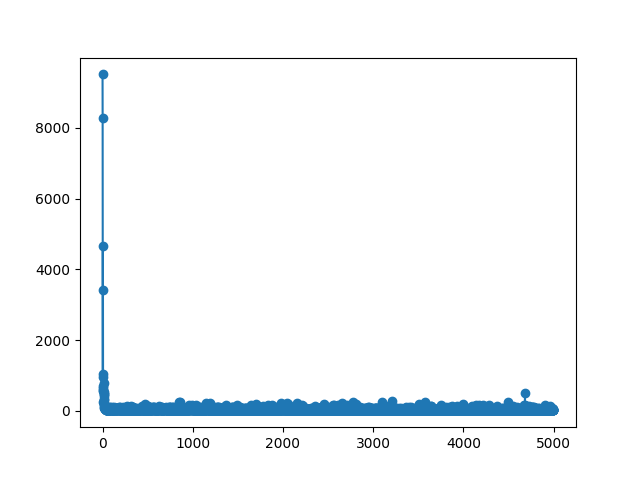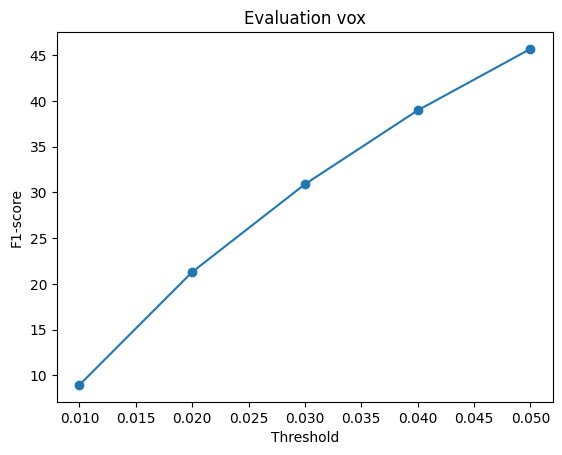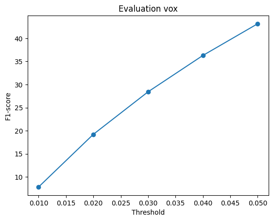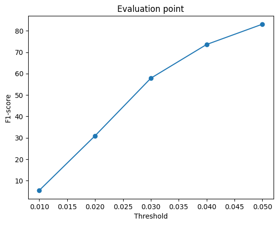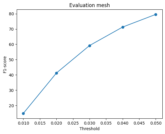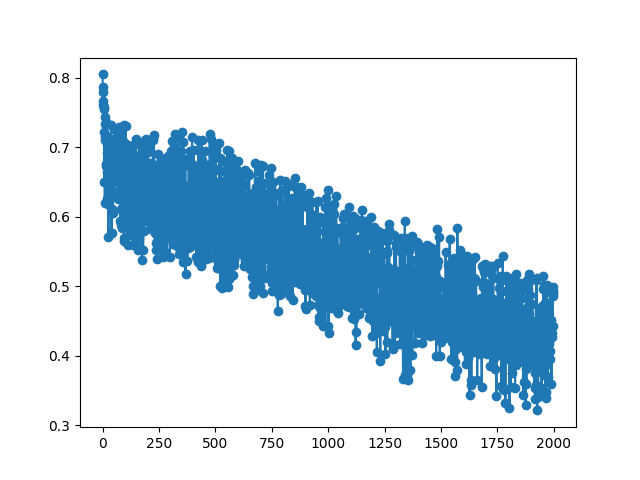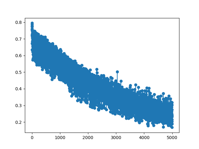Loss Curves ------------------------ ### Training Loss Curves for Voxels   ### Training Loss Curves for Point Clouds   ### Training Loss Curves for Mesh   Analyse Effects of Hyperparms Variations ------------------------ ### F1-Score Plot of Voxel Grid   ### F1-Score Plot of Point Cloud   ### F1-Score Plot of Mesh   **Explanation :** The hyperparameter "n_points" was modified and a performance comparison between two settings: n_points=5000 and n_points=10000 was conducted . The plots reveal that increasing n_points from 1000 to 5000 leads to a slight improvement in the model's F1-score, and the performance curves exhibit a smoother and more linear behavior. However, when n_points is further increased from 5000 to 10000, there is virtually no change in the F1-score. This could be attributed to the fact that 5000 n_points already provide sufficient information for the point cloud to yield good results, and increasing n_points beyond this threshold doesn't significantly impact performance. In such cases, it may be necessary to explore adjustments in other hyperparameters to enhance overall performance such as changing w_chamfer, vox_size, number of iterations and so on. 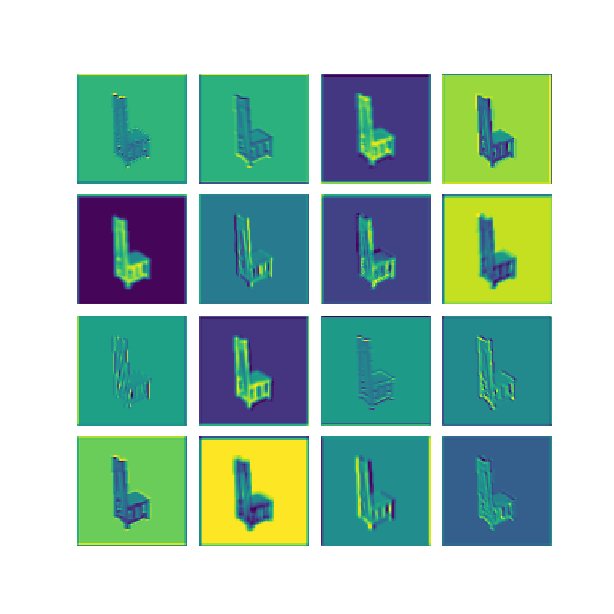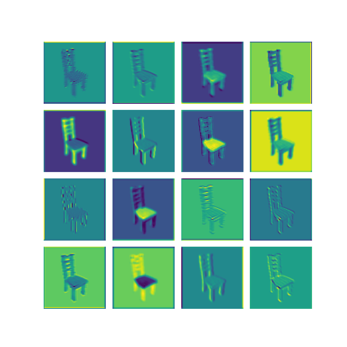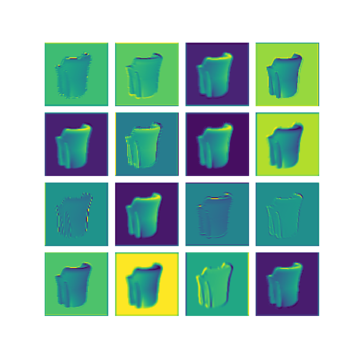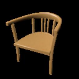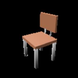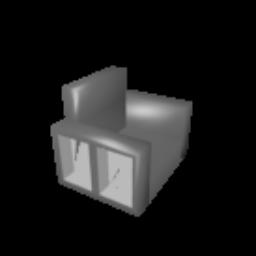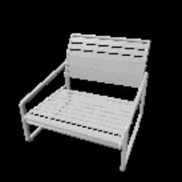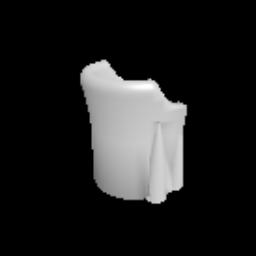Interpret Your Model ------------------------          **Explanation :** In this visualization, we are focusing on the activations of the second-to-last layer within the neural network's encoder. Our primary goal was to gain insights into how the model transforms and stores information derived from the input data. This visualization has provided us with a clear understanding of how the ResNet model has encoded features from the input information. Upon close examination of the visual results showcased above, it becomes evident that the encoder has effectively captured the general shapes and outer boundaries of the input objects. However, it is important to note that the encoder has limitations when it comes to recognizing intricate or finely-detailed aspects of the input. This particular constraint could potentially have a detrimental effect on the model's performance, especially in tasks related to predicting Meshes. It might struggle to accurately preserve the fine details inherent in the data, which is a critical aspect of certain applications. References ================ [848F-Assignment 1 Repository](https://github.com/848f-3DVision/assignment2) : Used for the README file and starter code. [PyTorch Official Documentation](https://pytorch.org/) [Pytorch 3D documentation](https://pytorch3d.org/)